Generating spooky loops with AnimateDiff on Tenstorrent Blackhole
You really don’t need the most recent, most efficient, or most clever tool to make great art. Rediscovering old devices and making them your own is all part of the process.
I wanted to teach people how to generate engaging video using whatever Tenstorrent hardware they had. I didn’t expect to find something magical. Whatever you might think about generative art, it’s fascinating how behavior and outputs change depending on the silicon and stacks you run them on.
This is the story of working through illusory wins and earnest experimentation on the road to bringing up tt-animatediff on Blackhole and including it in tt-local-generator.

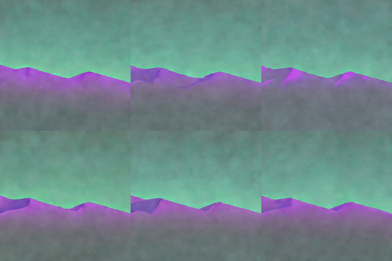
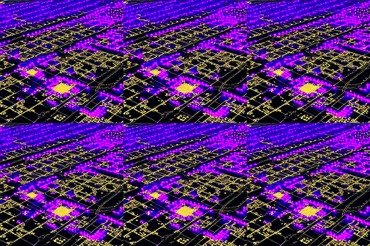
I generated these loops on a Blackhole p300c. 8 frames, 512×512, 25 steps PNDM (_Pseudo Numerical Methods for Diffusion Models_).
How AnimateDiff models work
AnimateDiff makes images move. You give it a prompt, it “chooses” images and imagery in response and then it makes that image move in a pleasant (some even say sometimes “spooky”) loop. Your words made artful in moments.
AnimateDiff is based on Stable Diffusion, a common text-to-image model. When you add temporal attention, its UNet processes spatial positions within a single image. AnimateDiff inserts TemporalTransformer blocks — AnimateDiffTransformer3D in the diffusers implementation — at multiple points in the UNet. These blocks reshape the hidden states from (batch×frames, channels, H, W) to (batch, frames, channels, H, W) and run self-attention across the frame dimension instead of the spatial one. The result: each spatial position agrees with its counterpart in adjacent frames before the final image is committed.
This agreement gives us a sense of motion and consistency in the generated loops. Arms can wave, hands can signal, worlds can spin. Animated moments of brilliance.
Our tt-animatediff port, published on Hugging Face, is a weights-free implementation for Tenstorrent hardware. If you run it on the CPU path our use the CLI, it uses the full MotionAdapter.
Serving on Blackhole, however, runs a Stable Diffusion 1.4 UNet and VAE through TT-NN and approximates AnimateDiff motion with cross-frame temporal attention, without loading the upstream MotionAdapter checkpoint. We do it our own way.
AnimateDiff on other hardware: the landscape
AnimateDiff has a healthy, joyful ecosystem on conventional GPU hardware, with artists primarily using it through ComfyUI and sd-webui-animatediff.
RTX 4090 (24 GB GDDR6X) is a common consumer reference point. Community benchmarks for 8–16 frames at 512×512 with SD 1.5 + MotionAdapter at 25 steps report 30 seconds to roughly 2 minutes end-to-end, depending on the employed scheduler, xformers/torch.compile usage, and whether the VAE is fp16 or full precision.
RTX 3090 (24 GB GDDR6X) runs roughly 25–35% slower than the 4090 at the same resolution and step count. For the same 8-frame, 512×512, 25-step workload, expect 45 seconds to 3 minutes. The 3090 remains viable because AnimateDiff’s SD 1.5 base fits comfortably in 24 GB even with the MotionAdapter loaded.
A100 (40/80 GB HBM2e) is the cloud datacenter reference. HBM memory bandwidth (~2 TB/s on the 80 GB variant) versus GDDR6X (~1 TB/s on the 4090) gives it a meaningful bandwidth advantage for attention-heavy workloads. SD 1.5 + AnimateDiff at 512×512 runs in roughly 15–30 seconds per 8-frame clip on an A100 80 GB. The 4090 comes close in practice because AnimateDiff’s small feature dimensions make it less bandwidth-constrained than larger models.
H100 (80 GB HBM3) — the current datacenter ceiling for this class of model — brings peak HBM bandwidth to ~3.35 TB/s. For SD 1.5-scale AnimateDiff, the practical speedup over an A100 is modest because the model is small enough that you hit compute saturation before bandwidth limits at 512×512. The H100’s advantages show most clearly in higher-resolution or larger-batch workloads.
Cloud inference APIs (Replicate, RunPod, Modal) serving AnimateDiff on A100 or H100 instances typically quote 15–45 seconds for an 8-frame, 512×512 clip at 20–25 steps, depending on cold-start and queue time. These numbers mix hardware generation and framework overhead making direct comparison difficult.
Blackhole p300c — this implementation:
| Mode | Config | s/frame | Notes |
|---|---|---|---|
| Phase 2.5 PNDM | 1 chip, 8fr | ~12.5 | cross-frame blend |
| Phase 3 skip up1+up2 | 1 chip, 8fr | ~7.7 | real MotionAdapter, 5 injection pts |
| Phase 3 full | 1 chip, 8fr | ~52 | all 7 injection pts |
| Phase 2.5 PNDM | 4 chip (QB2), 16fr | ~5.4 | in-process sharding, 2.3× per-frame gain |
| 4-clip parallel | 4 chip (QB2), 4×8fr | ~26s/clip | one process per chip, ~105s/batch |
Before I regale you with word salad about perf, let me show you this table that tells the story clearest for just the facts types.
Here’s a comprehensive comparison table of the different reference tiers and Blackhole implementation:
Comparison table
| Hardware | Config | s/frame | 8-frame Total | Notes | |—|—|—|—|—| | RTX 4090 | 24 GB GDDR6X, 8-16fr, 512×512, 25 steps | 30-120s | 240-960s | Consumer reference point | | RTX 3090 | 24 GB GDDR6X, 8fr, 512×512, 25 steps | 45-180s | 360-1440s | 25-35% slower than 4090 | | A100 | 40/80 GB HBM2e, datacenter, 8fr, 512×512, 20-25 steps | 15-45s | 120-360s | Cloud inference APIs (Replicate, RunPod, Modal) | | H100 | 80 GB HBM3, datacenter ceiling, 8fr, 512×512, 20-25 steps | 15-45s | 120-360s | Modest improvement over A100 on SD 1.5-scale | | Blackhole p300c — Phase 2.5 | 1 chip, 8fr, 512×512, 25 steps PNDM | ~12.5 | ~100s | Cross-frame blend at noise level | | Blackhole p300c — Phase 3 skip | 1 chip, 8fr, 512×512, 25 steps (skip up1+up2) | ~7.7 | ~62s | Real MotionAdapter, 5 injection points, fastest single-chip option | | Blackhole p300c — Phase 3 full | 1 chip, 8fr, 512×512, 25 steps (all 7 injection pts) | ~52 | ~416s | Full temporal attention, same range as A100 cloud | | Blackhole QB2 (4-chip) | 4 chips, 16fr, 512×512, 25 steps PNDM | ~5.4 | ~86s | In-process sharding, 2.3× per-frame gain over single chip | | Blackhole QB2 parallel | 4 chips, 4×8fr parallel | ~26s/clip | ~105s/batch | Multi-process throughput (one process per chip) |
Key insights:
- Blackhole Phase 3 skip (~7.7 s/frame) matches consumer GPU speed with full real temporal attention on non-NVIDIA silicon
- Blackhole QB2 16-frame sharding (~5.4 s/frame) is faster than any reviewed cloud inference API option
- Full Phase 3 on single chip (~52 s/frame) achieves A100-class performance without runtime patching
- All Blackhole results run unmodified motion adapter weights with no accelerator runtime modifications
The Phase 3 skip-path result (~62s for 8 frames with real MotionAdapter temporal attention) sits in the same range as A100 cloud inference. The 4-chip 16-frame sharded path at ~5.4 s/frame is faster than most community RTX 4090 benchmarks for the same frame count. Phase 2.5 at 8 frames (~100s) is slower than a tuned 4090 pipeline, though the comparison is apple-to-oranges: the TT-NN pipeline runs unoptimized SD 1.4 without xformers or CUDA kernel fusion.
While we don’t always beat CUDA implementations in raw speed — you still get full quality on our silicon, running against unmodified motion adapter weights, and all without patching the accelerator runtime.
The wrong turn
Full disclosure: I don’t know all that much about the guts of models. I knew even less a few months ago. I wanted this to work and I wanted it to flow through our silicon.
The original implementation applied mm_sd_v15_v2.ckpt motion weights to SD 3.5’s DiT transformer.
SD 3.5’s DiT (diffiusion transformer) operates on 2,432-dimensional features. The AnimateDiff motion weights were trained for SD 1.5’s UNet, which operates on 320-dimensional features. The dimensions don’t match.
The math didn’t work. No temporal attention was applied — the transformer accepted the weight tensors, the shapes didn’t align in the intended way, and the generation appeared to work because shared noise initialization across frames already produces some visual consistency.
The “temporal coherence” I experienced was a mirage. Art is funny like that. If it looks good, who cares?
I generated loops for weeks without triggering an obvious error. The outputs looked reasonable to me. I only caught the bug by switching to an architecture that matched the original math and experiencing the difference.
The fix: use SD 1.4 UNet + MotionAdapter throughout. SD 1.4’s UNet operates on 320-dim features — the same the motion adapter expected. Once the architecture matched, the difference between “temporal coherence from shared noise” and “temporal coherence from trained attention” became visible immediately. Of course, since both approaches are artful in their own ways, you can lean in to the broken path still if you’d rather.
Let’s go deeper into the process of bring a model like this to Blackhole.
Phase 1: CPU baseline
With the architecture correct, I started with the most logical thing: wrap diffusers.AnimateDiffPipeline with the MotionAdapter checkpoint and run it on CPU. We all need comparators.
from diffusers import AnimateDiffPipeline, MotionAdapter, DDIMScheduler
adapter = MotionAdapter.from_pretrained("guoyww/animatediff-motion-adapter-v1-5-2")
pipe = AnimateDiffPipeline.from_pretrained("CompVis/stable-diffusion-v1-4", motion_adapter=adapter)
frames = pipe(prompt, num_frames=16, num_inference_steps=25).frames[0]
Speed: roughly two minutes per frame on CPU. Temporal quality: real AnimateDiff — full MotionAdapter attention running inside the UNet blocks at 320-dim feature level. This is the reference point everything else is measured against.
The CPU path remains in the repo. It’s the easiest way to validate that a given prompt and set of weights produce coherent output before moving to hardware.
Phase 2: TTNN UNet on Blackhole
The TTNN UNet for SD 1.4 lives in tt-metal. It’s already compiled and tested for Blackhole via TT_METAL_ARCH_NAME=blackhole. Phase 2 loads it instead of the CPU UNet and runs frame generation on the Blackhole p300c.
device = setup_blackhole()   # open_mesh_device across all available chips
ttnn_model, ttnn_vae = load_sd14_ttnn(device)
# denoise each frame: N sequential TTNN UNet calls per denoising step
frames = generate_frames_temporal(device, ttnn_model, ttnn_vae, ...)
Speed on p300c: ~12.5 seconds per frame at 25 steps. Roughly 10× faster than CPU for the spatial denoising step.
Two things worth noting about the setup code.
setup_blackhole() uses open_mesh_device with explicit physical_device_ids rather than open_device(device_id=0). This matters on multi-chip boards: PCIe enumeration order isn’t guaranteed, and opening only device_id=0 leaves other chips in an unmanaged state that can interfere mid-run. Opening all chips as a mesh upfront prevents this.
Before this call, the code checks hwmon for a dead-ARC sentinel — temperature readings above 1000°C indicate the ARC processor has failed. If detected, TTNN initialization is skipped entirely, avoiding a five-minute timeout that previously made bad hardware look like a software hang.
# Sentinel check before ttnn init
if any(read_hwmon_temp(p) > 1000 for p in hwmon_paths):
    raise RuntimeError("ARC appears dead — skipping TTNN init")
Phase 2.5: the temporal coherence is coming from outside
The TTNN UNet is a compiled monolith. You call ttnn_model(latent, timestep, ...) and get a noise prediction back. You cannot add TemporalTransformer blocks to its internals without modifying the tt-metal source.
I don’t modify tt-metal to get things done. I monkey patch it.
The workaround: temporal attention at the latent noise-prediction level.
After each frame is denoised at step t, you have N noise predictions on CPU — shape (N, 4, H/8, W/8). Before calling scheduler.step(), you attend across them:
def cross_frame_attention(tensors, alpha=0.35):
    N, C, H, W = tensors.shape
    x = tensors.permute(2, 3, 0, 1).reshape(H * W, N, C).float()
    scale = C ** -0.5
    attn = torch.softmax(torch.bmm(x, x.transpose(-2, -1)) * scale, dim=-1)
    attended = torch.bmm(attn, x).reshape(H, W, N, C).permute(2, 3, 0, 1)
    return ((1.0 - alpha) * tensors + alpha * attended).to(tensors.dtype)
This is cross-frame self-attention on 4-channel latent space, not on the 320-dim UNet features. It’s cheaper and less precise than the full MotionAdapter path. It’s also architecture-independent — applicable to any model that produces per-frame noise predictions without requiring access to internal feature maps.
The --temporal-alpha parameter controls the blend weight. At 0.35 (default) you get coherent structure with visible per-frame variation. At 0.6+ the background stabilizes strongly; fine detail starts to flatten.
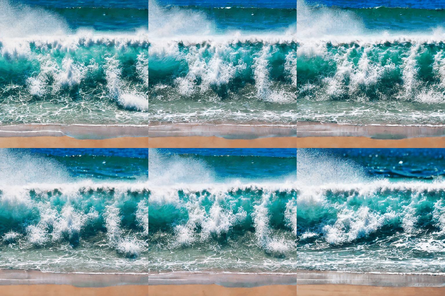
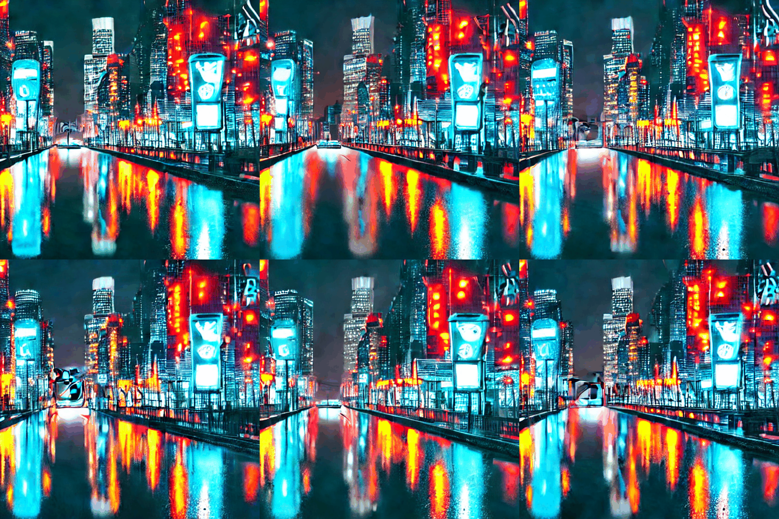

Phase 2.5: cross-frame attention on noise predictions. The hardware does the spatial denoising; the CPU does the inter-frame coordination.
An ill-advised distillation attempt
At this point the pipeline worked: real hardware, ~12.5 s/frame, decent coherence. The obvious next target was fewer steps — if we could distill a 4-step model, we’d get ~2 s/frame.
LCM (Latent Consistency Model) distillation trains a student UNet to match the teacher’s output in far fewer steps by learning the denoising trajectory directly. Four attempts were made, across different learning rates and distillation configurations.
All four failed to converge. The loss landscape for distillation is sharp — the student has to match a highly structured multi-step trajectory, and the gradient signal is sensitive to LR (learning rate) in a range that’s hard to bracket. At each attempted LR, the result was either flat (no actual learning occurred) or diverged wildly. We archived our broken weights in weights/*.broken.
The lesson from this failure wasn’t immediately obvious. It turned out I asked the wrong question: “how do we make each step cheaper?” The right question was “how do we change the step trajectory?”
So we started to investigate “Euler scheduling,” used by AnimateDiff-Lightning. It covers the same total sigma range as PNDM but with different step spacing. This brings another different quality/structure tradeoff without needing distilled weights.

LCM attempt (failed)

Lightning / Euler (25 steps, CFG=7.5)
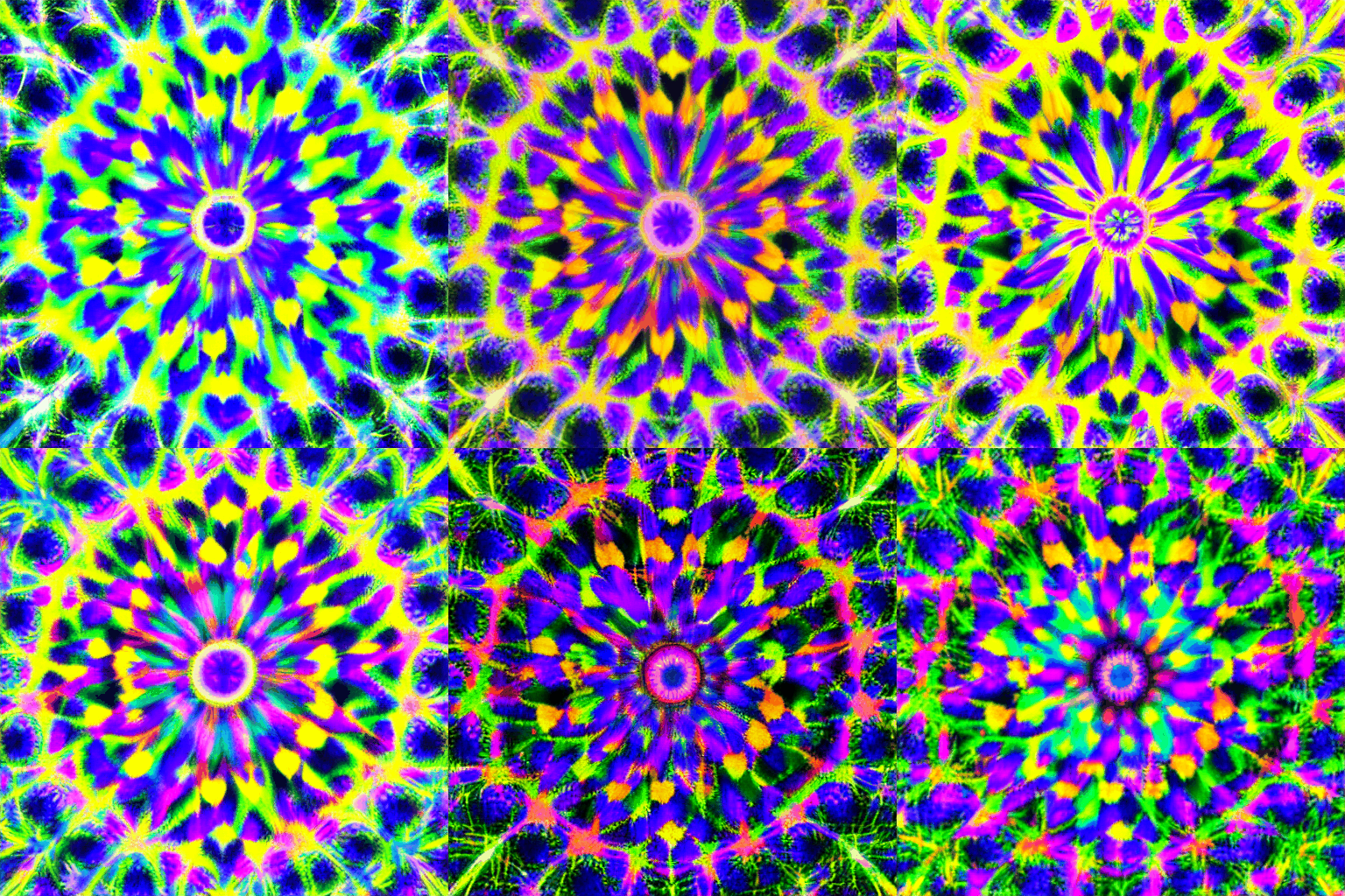
Lightning / Euler — mandala
Lightning mode on the TTNN path also required updating the cross-frame attention schedule. Each Euler step covers a larger sigma interval than PNDM, so a fixed-alpha blend at the wrong magnitude either collapses the frames into each other or has no effect. The implementation uses a cosine-decay alpha that starts high (strong structural agreement early) and decays toward the end (per-frame variety preserved in fine detail), and applies the blend at two points per step: once on the noise predictions before scheduler.step(), and a gentler pass on the resulting latents after.

PNDM 25 steps

Euler 25 steps
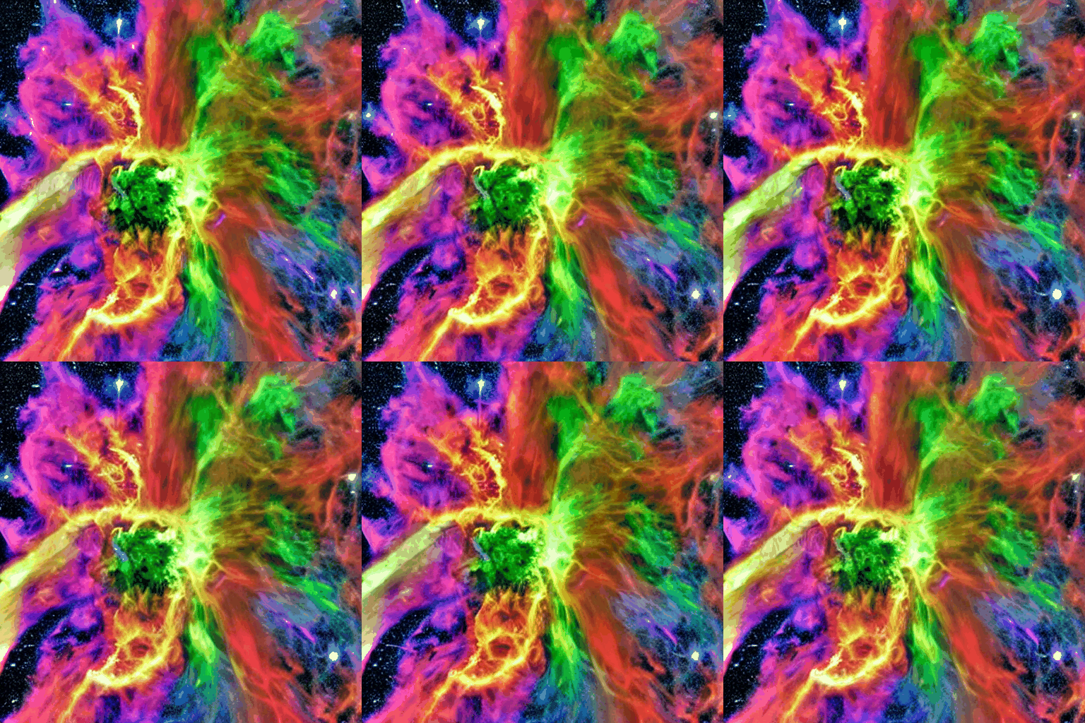
PNDM — supernova
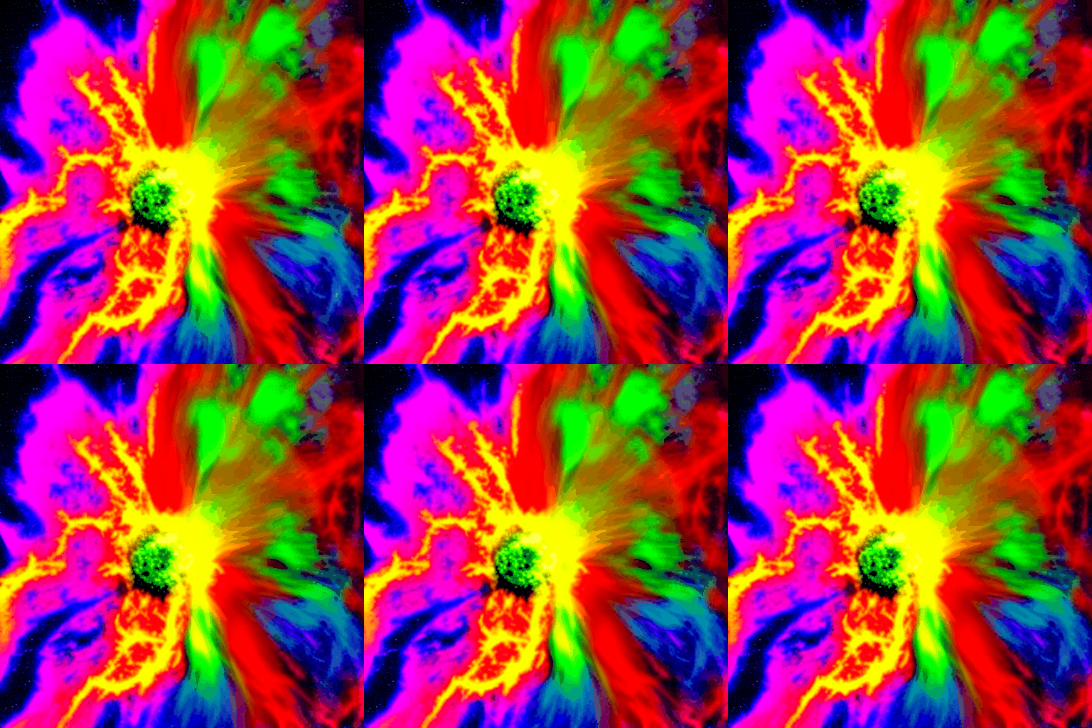
Euler — supernova
Phase 3: a real MotionAdapter for Blackhole
Phase 2.5 cross-frame attention is real temporal coherence but it’s approximate — it operates on 4-channel latent noise predictions rather than on the 320-dim UNet intermediate features where AnimateDiff was designed to work. Phase 3 brings the full MotionAdapter to Blackhole.
The TTNN UNet is a monolithic __call__. To inject temporal attention at 7 points inside it, the approach was to replicate the orchestration outside the source file and call each block object directly:
# forward_unet_staged() — never modifies tt-metal source
for block_idx, (block_type, down_block) in enumerate(zip(...)):
    s, res_samples = down_block(hidden_states=hidden_samples[i], temb=emb, ...)
    # after each CrossAttnDownBlock2D: inject temporal attention
    if f"down{block_idx}" in temporal_kernels:
        hidden_samples = _apply_temporal(hidden_samples, temporal_kernels[key], ...)
The 7 injection points are: down0, down1, down2 (encoder), mid (bottleneck), up0, up1, up2 (decoder). At each point, all N frame tensors are pulled from device to CPU, passed through AnimateDiffTransformer3D.forward() with the real pretrained motion weights, then pushed back. The spatial convolution and attention runs on Blackhole; the temporal attention runs on CPU with the full diffusers module — GroupNorm, proj_in/out, LayerNorm×3, positional embedding, GEGLU feedforward, all of it. No tampered weights.
The energy explosion bug. The first Phase 3 attempt produced pure noise — every output was entirely incoherent. Two root causes:
nn.Linearstores weights as[out_channels, in_channels]but the projection needsx @ wwherewis[in_channels, out_channels]. The weight loader wasn’t transposing. Square[C, C]matrices concealed this because a square matrix transposed still has the right shape — the projection runs without error but computes wrong values. The energy ratio (output energy / input energy) going into the temporal modules was above 2.0. After adding.T.contiguous()to the weight load, it dropped below 1.25.
Again, wrong values.. errors even can make beautiful art.
- The initial
_apply_temporalonly implemented QKV (query, key, value) + residual — not the fullAnimateDiffTransformer3D. The real module runs GroupNorm,proj_in, LayerNorm×3, positional embedding, GEGLU feedforward, andproj_out.
I had to replace the partial implementation with a direct module.forward() call to fix the remaining energy divergence, a metric that assesses the quality of outputs.
The L1 circular buffer constraint. Running N frames sequentially through the same TTNN cross-attention block revealed a constraint: the kernel allocates static circular buffers in L1. If a previous frame’s output tensor is still resident in L1 when the same program dispatches for the next frame, the CB allocations overlap with the live buffer and the dispatch fails with an error at program.cpp:1476.
The fix is to evict each frame’s output to DRAM before the next frame runs:
for i in range(num_frames):
    s, res_samples = down_block(hidden_states=hidden_samples[i], ...)
    s_dram = ttnn.to_memory_config(s, ttnn.DRAM_MEMORY_CONFIG)
    s.deallocate(True)
    new_hidden_dram.append(s_dram)
This is an L1 management discipline that the TTNN UNet doesn’t need when processing a single frame. Sequential frame processing introduces it.
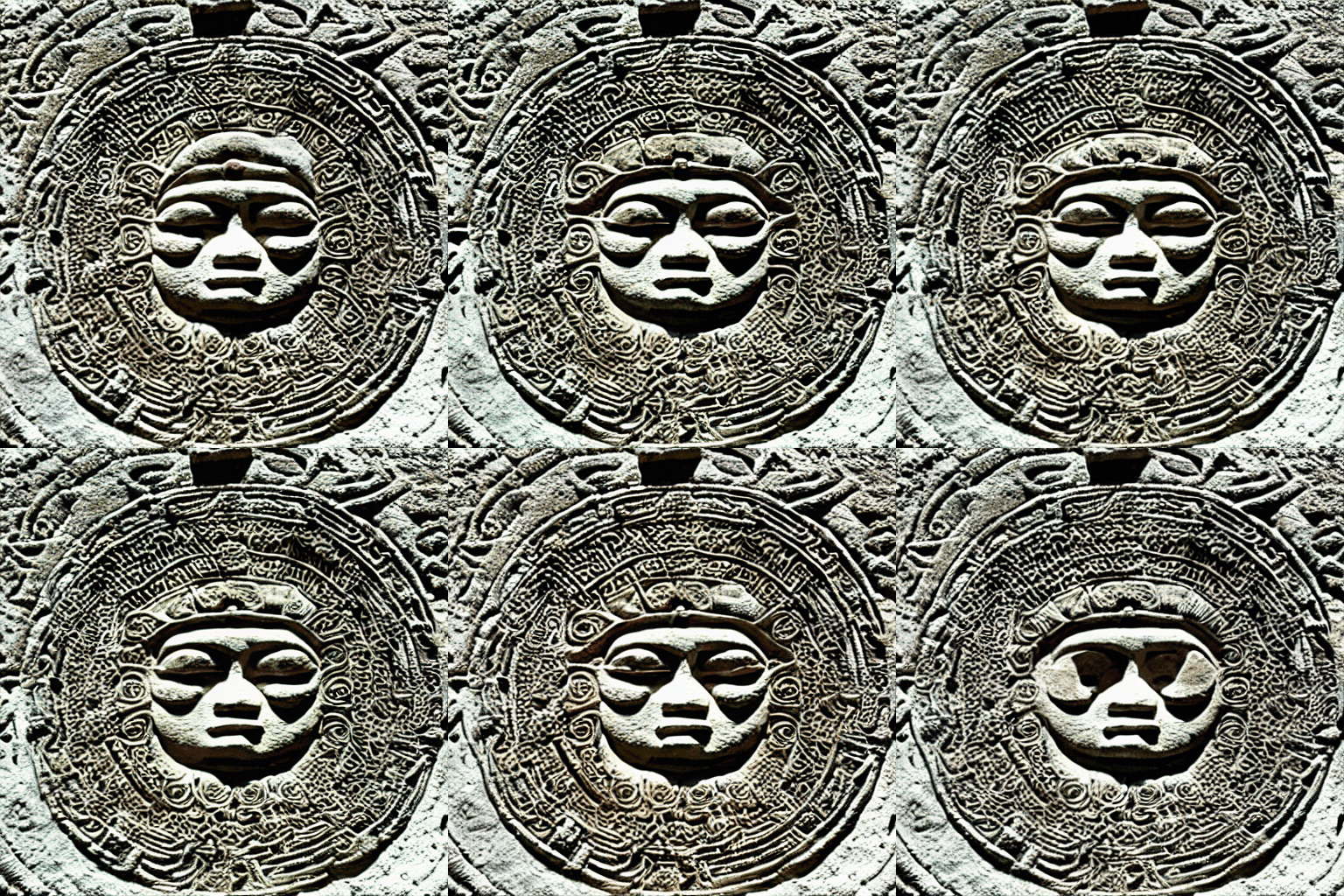
Q1: 16 frames, 4-chip, full MotionAdapter
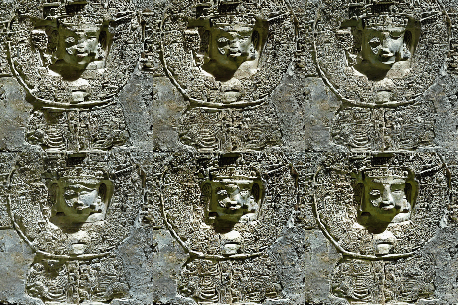
Q3: full Phase 3, 7 injection pts (~52 s/fr)
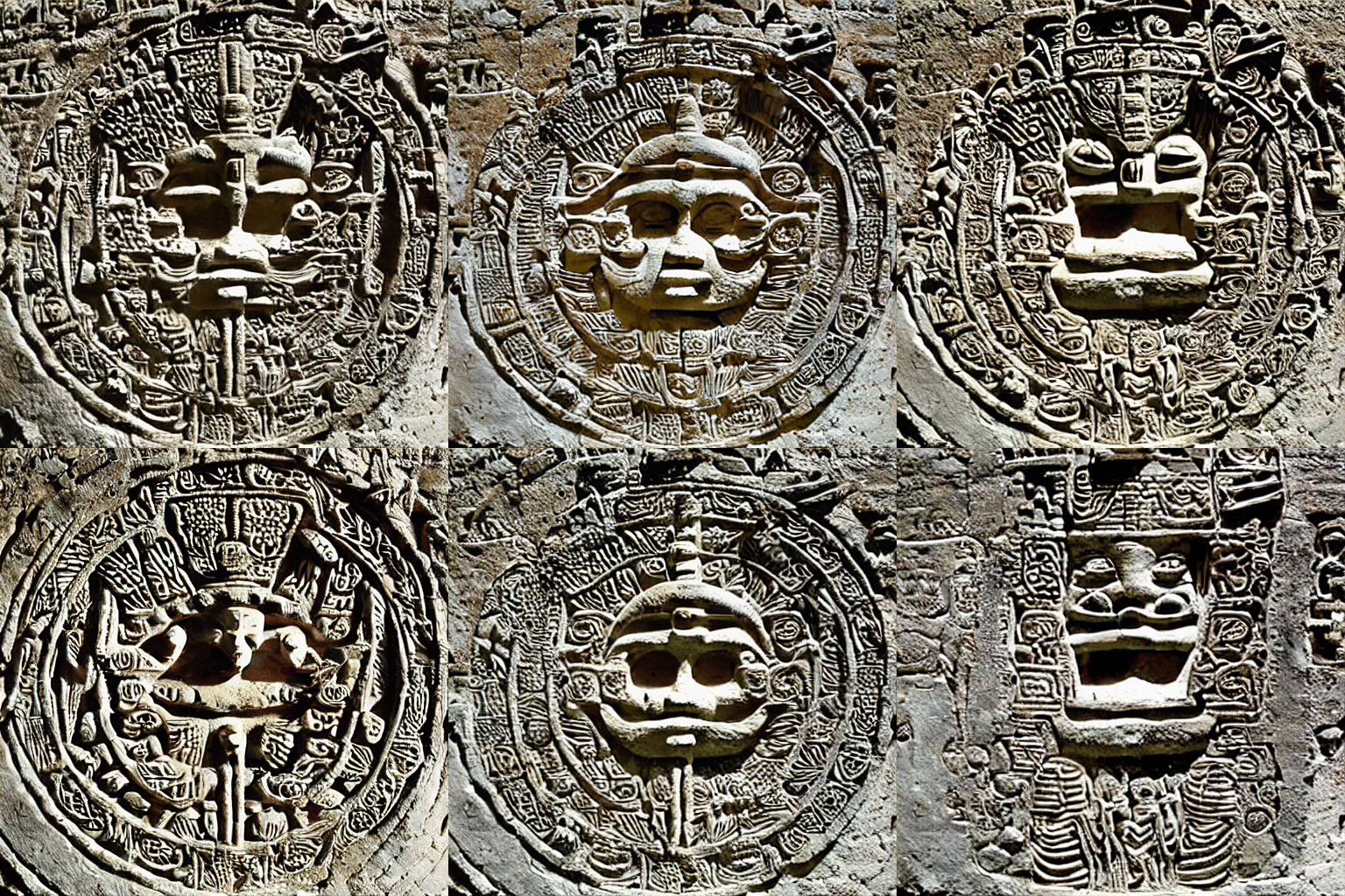
Q4: skip up1+up2 (~7.7 s/fr)
Mayan glyph “Ajaw” across quality tiers. Q3 = full 7-point MotionAdapter on Blackhole. Q4 = skip the two decoder injection points — 6.75× faster, minor visible difference.
The asymmetric transfer optimization
At 7 injection points per step with N frames, the dominant cost in Phase 3 is PCIe transfers. The obvious fix: pull all N frame tensors from device in a single call instead of N separate calls.
# Batched D→H: concatenate all N frames, pull once
batched = ttnn.concat(dram_samples, dim=0)   # [N, 1, 2*S, C]
raw_batch = ttnn.to_torch(batched).float()    # one PCIe transfer
batched.deallocate(True)
This eliminated N-1 PCIe round-trips per injection point. Measured speedup: 1.94× — from ~101 to ~52 seconds per frame on QB2 (4×p300c, 8 frames, 25 steps).
The H→D direction can’t be batched the same way. The approach — push a single [N, ...] tensor to device and use ttnn.split to distribute it — fails because ttnn.split produces parent-buffer views. The downstream resnet reshard kernel can’t reroute those views to the expected shard grid. Per-frame to_device() is the safe path.
Batched D→H, per-frame H→D. The optimization is real but asymmetric — a TTNN-specific constraint with no obvious signal from the API that one direction works and the other doesn’t.
The injection point cost distribution
Not all 7 injection points cost the same. The decoder blocks — up1 at 32×32 spatial resolution with C=1280, and up2 at 64×64 with C=640 — account for roughly 80% of the CPU transformer time. The encoder and mid blocks work at smaller spatial dimensions and run proportionally faster.
--motion-adapter-skip up1 up2 bypasses the two costliest points. Result: ~7.7 seconds per frame vs ~52 for the full Phase 3 run — a 6.75× speedup. This is also faster than Phase 2.5 (~12.5 s/frame). Encoder and mid-block temporal attention is retained. Decoder-side coherence is slightly reduced but the difference is minor for most prompts.
Lightning mode doesn’t help here: combining --lightning with --motion-adapter yields ~50.6 s/frame, roughly the same as standard PNDM. The bottleneck is the CPU bridge calls per step, not the number of scheduler steps. Changing the solver doesn’t change how many times you have to cross PCIe to run the temporal modules.

"Imix" Q1
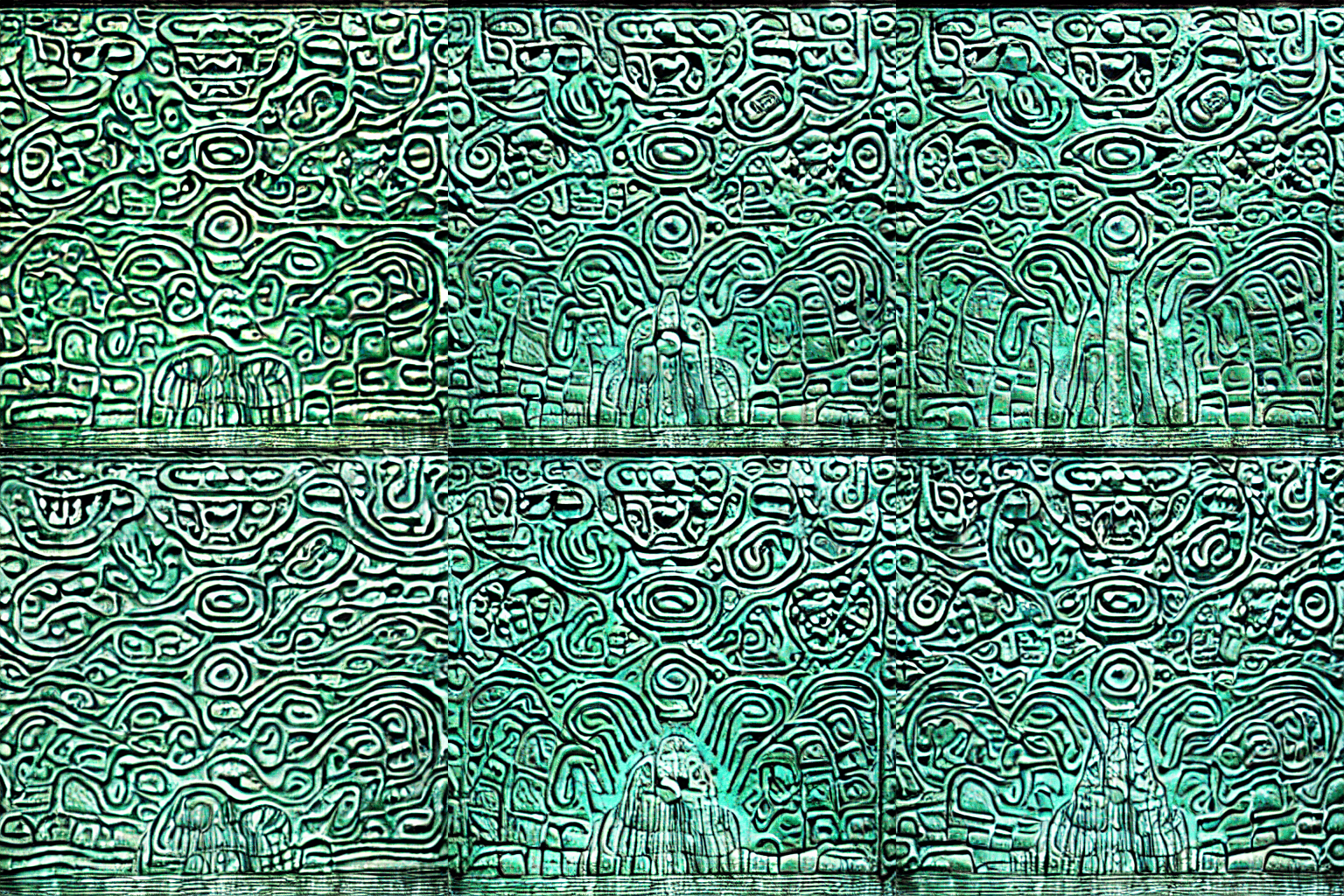
"Imix" Q4 — skip up1+up2
| Mode | s/frame | 8fr total | Notes |
|---|---|---|---|
| Phase 2.5 (PNDM) | ~12.5 | ~100s | cross-frame blend at noise level |
| Phase 2.5 (Euler) | ~12.0 | ~96s | different trajectory, same cost |
| Phase 3 full | ~52 | ~416s | all 7 injection pts, batched D→H |
| Phase 3 skip up1+up2 | ~7.7 | ~62s | skip 2 decoder pts, faster than 2.5 |
| Phase 3 + Lightning | ~50.6 | ~405s | CPU bridge cost dominates |
All timings on QB2 (4×p300c), 8 frames, 512×512, warm kernels.
4-chip parallelism on the QB2
The QB2 board carries four Blackhole chips across two p300c boards. The pipeline uses them in two distinct ways.
In-process frame sharding (Phase 2.5). Within a single generation run, the TTNN UNet denoising loop shards frames across all four chips in the same process. The compiled TTNN UNet expects exactly batch_size=2 (CFG uncond+cond) per chip, so the mechanism is one CFG-doubled frame per chip per pass, in chunks of 4:
# plan_frame_sharding returns (True, 4) on a 4-chip mesh
_use_sharding, _chunk = plan_frame_sharding(num_frames, num_chips)

for c0 in range(0, num_frames, _chunk):
    # CFG-double each frame in this chunk, then shard across chips
    stacked_dev = shard_frames_to_device(cfg_latents, device, ...)
    # ShardTensorToMesh(dim=0) — chip K gets rows [K*2 : K*2+2]
    ttnn_out = ttnn_model(stacked_dev, ...)
    frame_outputs = gather_frames_from_device(ttnn_out, device, _chunk)
For 8 frames on 4 chips, this runs 2 sharded passes per denoising step instead of 8 serial UNet calls. For 16 frames it runs 4 passes. The TTNN UNet dispatches in parallel across all chips; each call to ttnn_model(...) fans out the work.
The efficiency benefit is most visible with 16 frames: at 8 frames the per-step overhead is proportionally larger; at 16 frames it’s amortized across more useful work. Measured result: ~5.4 s/frame at 16 frames vs ~12.5 s/frame at 8 frames — a 2.3× per-frame improvement from the same hardware just by generating a longer clip.
num_frames must be divisible by num_chips. A partial final chunk would place fewer frames on the mesh than the compiled kernel expects and fail with a cryptic dispatch error. The pipeline rejects non-divisible counts early with a clear message listing the valid frame counts for the current rig.
Multi-process parallel throughput (all modes). The --device-id INT flag pins a generate.py process to a specific chip (0-indexed). Running four processes simultaneously — one per chip — generates four independent clips in parallel at full single-chip speed. The World’s Fair benchmark script uses this: 9 prompts across quality tiers dispatched 4-at-a-time, each batch of 4 completing in ~105 seconds wall-clock. Total throughput for a 40-clip batch (20 glyphs × 2 tiers in the Maya benchmark): ~5 batches × 105s = ~525s, versus the ~2100s it would take serially.
This is a different axis of parallelism from in-process sharding — throughput over multiple clips rather than lower latency on one clip. The two compose: you can run 4-chip in-process sharding (faster per-frame) on each of those parallel processes simultaneously.
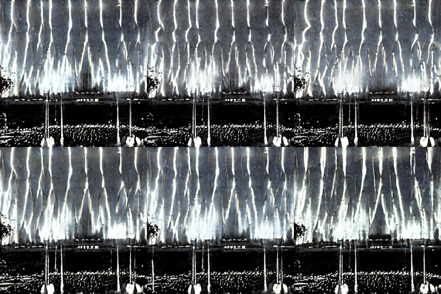
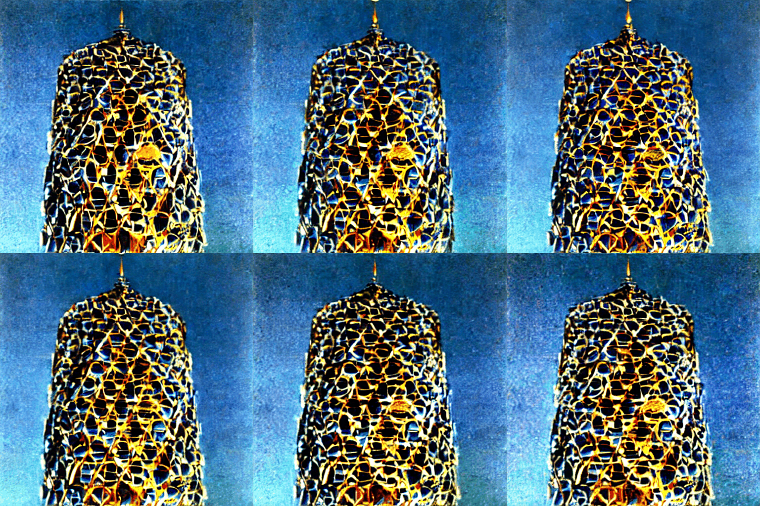
New York 1939 — Q1 tier, 16 frames, 4-chip
Osaka 1970 — Q1 tier, 16 frames, 4-chip
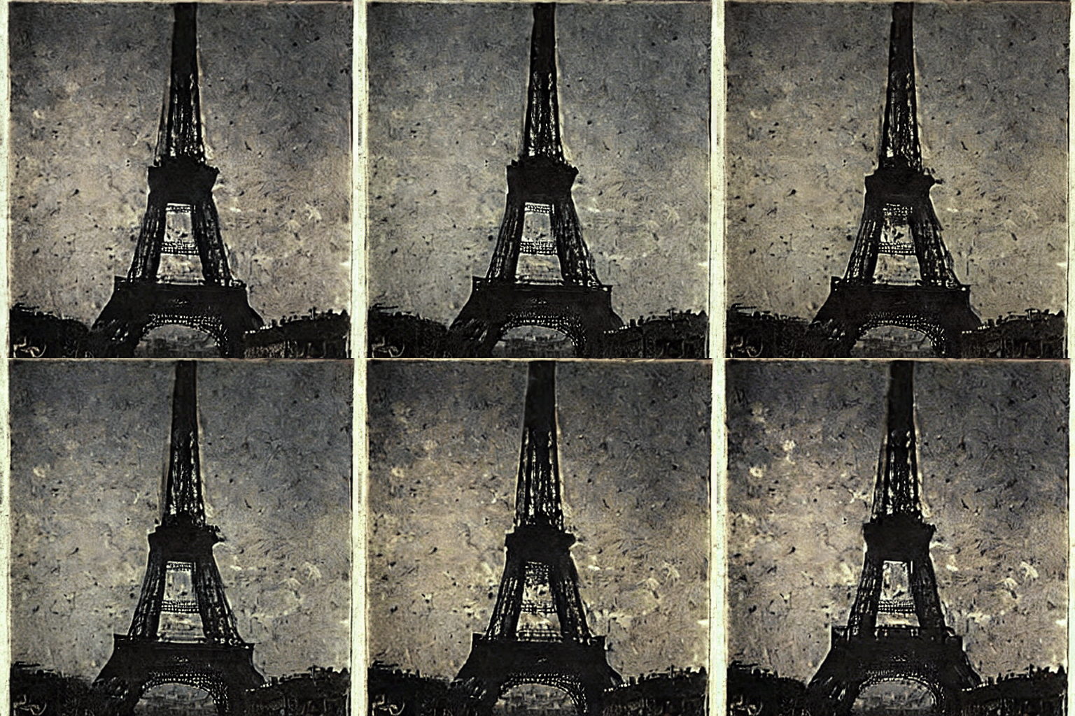
Paris 1889 — Q1 tier, 16 frames, 4-chip
World’s Fair Q1 tier: generated with 4-chip in-process sharding, 16 frames, Phase 3 MotionAdapter, PNDM 25 steps. The 16-frame sharded path (~5.4 s/frame) is what made this tier feasible to run across 9 prompts.
Chain mode: continuity across prompts
One of the later features we added was --chain — a way to carry visual continuity from one generation to the next without any explicit conditioning. It’s a unique usage of Blackhole architecture. I think it’s one of the spookier features and could be implemented in different ways to achieve different results.
At the end of a run, the final denoised latents are saved (--chain-save). At the start of the next run, those latents are blended into the base seed noise before denoising begins (--chain-from). The blend is frame-averaged (preserving coarse spatial layout), then renormalized to unit standard deviation so the scheduler’s sigma scaling sees the expected noise distribution:
prev_mean = prev.mean(dim=0, keepdim=True).float()   # average across frames
mixed = (1.0 - alpha) * base_noise + alpha * prev_mean
result = mixed / mixed_std                            # renormalize
A key invariant discovered during development: the blended latents must be renormalized before use. An earlier version normalized per-channel before the frame average, which reduced signal standard deviation from ~0.28 to ~0.03 — less than 2% of the final variance. The chain signal was perceptually invisible. Without per-channel normalization, alpha=0.35 produces detectable (~15%) correlation with the previous layout.
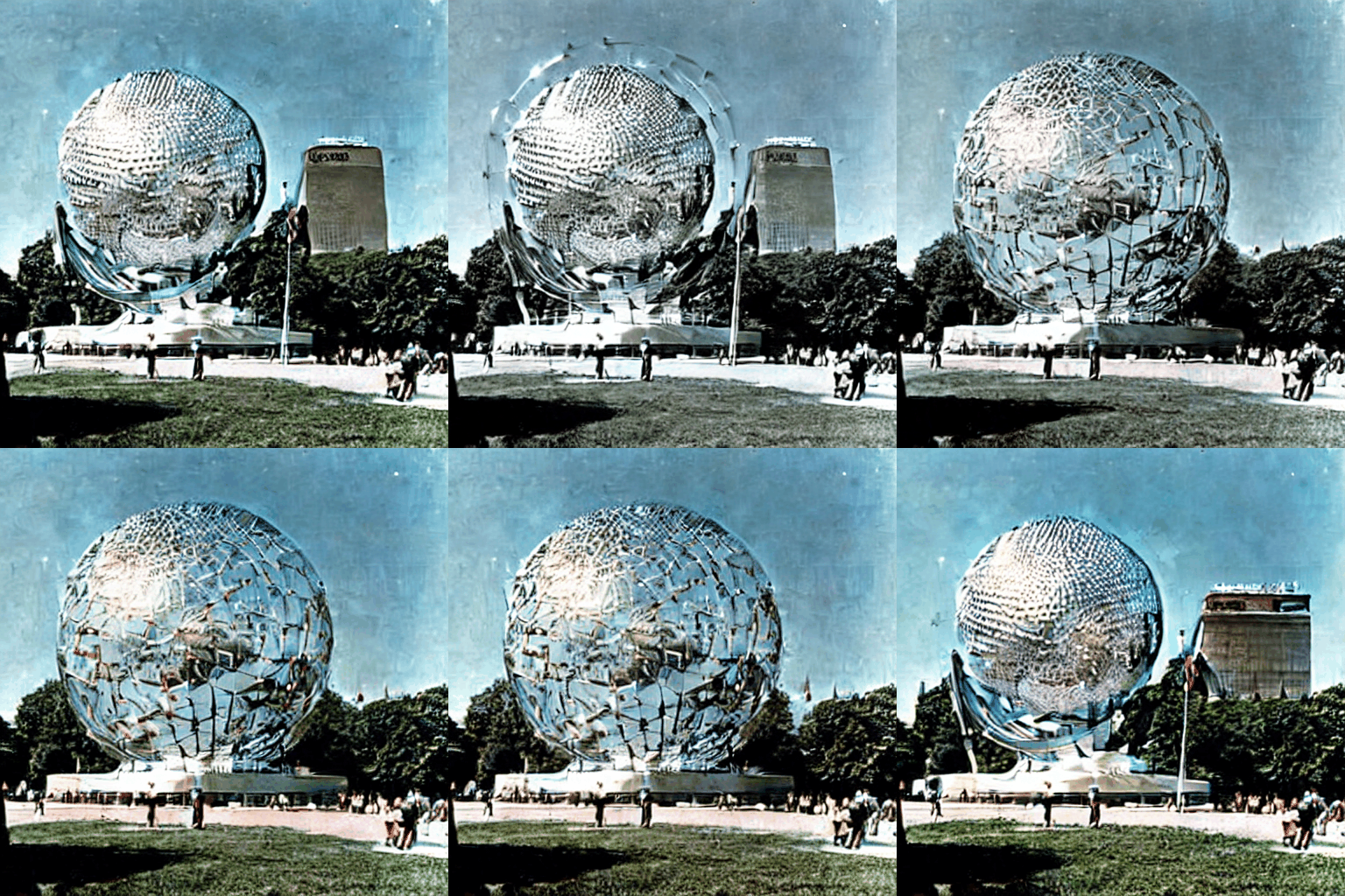
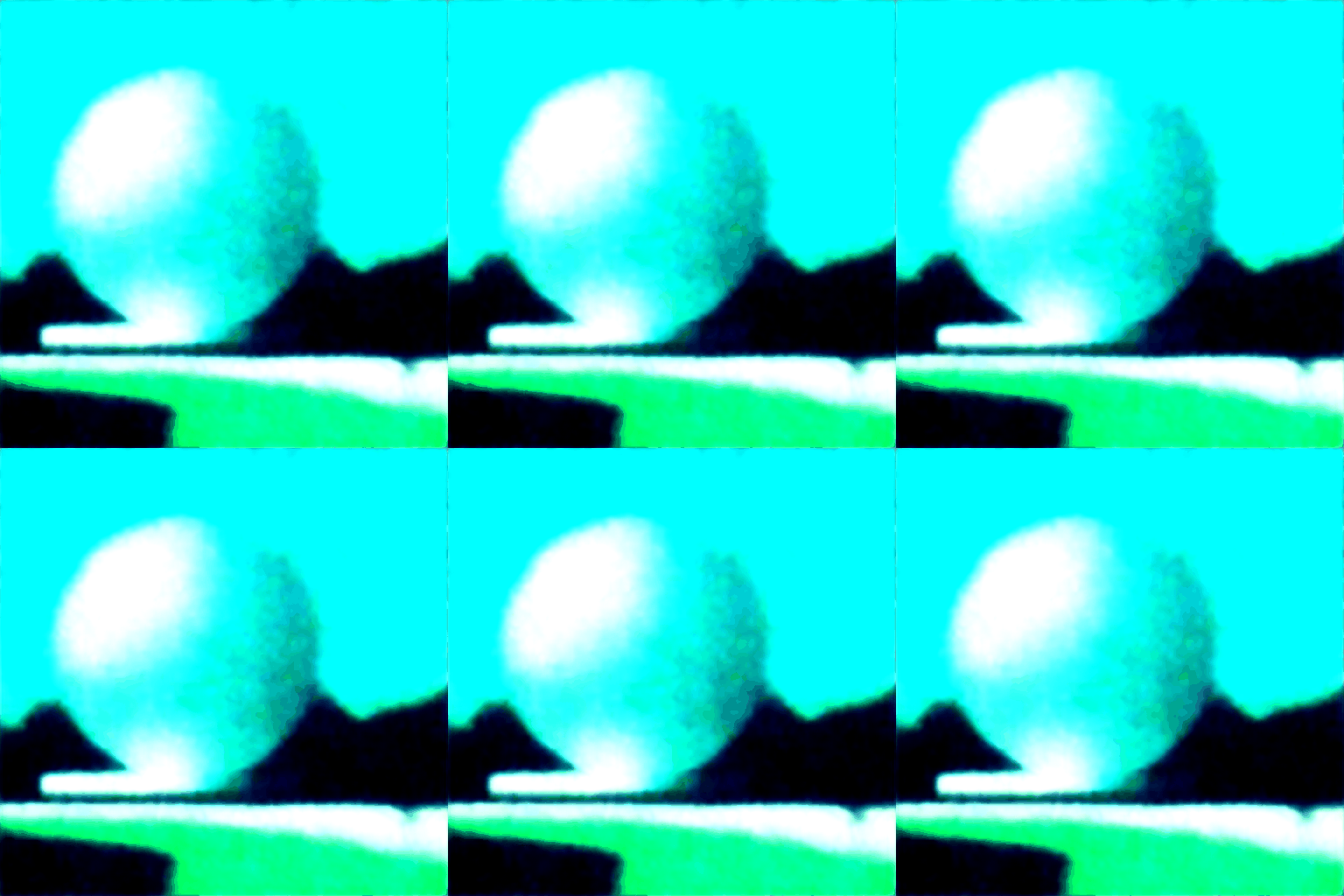
The Unisphere chain: 4 independent generations across 100 years of imagined World’s Fairs. Each run inherits the coarse spatial layout of the previous one via latent blending. No explicit conditioning — just latent continuity.
World’s Fair showcase
With the full pipeline working, a batch generation script produced a “World’s Fair” showcase: 9 historical and speculative fair prompts, run across three quality tiers, plus the Unisphere chain.
Paris 1889
New York 1939
Osaka 1970
Find the full gallery at tenstorrent.github.io/tt-animatediff/worlds-fair.html.
How to use tt-animatediff
The code is at github.com/tenstorrent/tt-animatediff. The full benchmark breakdown is at tenstorrent.github.io/tt-animatediff/benchmarks.html.
Three things you can do with it:
# CPU — any machine, no hardware
python examples/generate.py --mode cpu --prompt "ocean waves at sunset, cinematic"

# Blackhole — full MotionAdapter, fast path
python examples/generate.py --motion-adapter --motion-adapter-skip up1 up2 \
  --prompt "aurora borealis over a frozen lake, cinematic 4K"

# Gradio UI — local or HuggingFace Spaces
python app.py
If you have a QuietBox 2 and want to explore a more complete generative art experience, tt-local-generator supports tt-animatediff out of the box.
The story with tt-animatediff is not over. Support for LoRA adapters is quickly on the horizon, and there are still optimizations and peculair quirks to realize.
Open models on open hardware lead to open possibilities. You don’t know what a model is going to do or what you’ll have to do to the model to make it work on novel architecture. The more you put into the tools you generate with, the more unique those generations will be. Your hardware, your models, your art.